Symbolic circuits with pytket-qujax#
In this notebook we will show how to manipulate symbolic circuits with the pytket-qujax extension. In particular, we will consider a QAOA and an Ising Hamiltonian.
See the docs for qujax and pytket-qujax.
from pytket import Circuit
from pytket.circuit.display import render_circuit_jupyter
from jax import numpy as jnp, random, value_and_grad, jit
from sympy import Symbol
import matplotlib.pyplot as plt
import qujax
from pytket.extensions.qujax import tk_to_qujax
QAOA#
The Quantum Approximate Optimization Algorithm (QAOA), first introduced by Farhi et al., is a quantum variational algorithm used to solve optimization problems. It consists of a unitary \(U(\beta, \gamma)\) formed by alternate repetitions of \(U(\beta)=e^{-i\beta H_B}\) and \(U(\gamma)=e^{-i\gamma H_P}\), where \(H_B\) is the mixing Hamiltonian and \(H_P\) the problem Hamiltonian. The goal is to find the optimal parameters that minimize \(H_P\). Given a depth \(d\), the expression of the final unitary is \(U(\beta, \gamma) = U(\beta_d)U(\gamma_d)\cdots U(\beta_1)U(\gamma_1)\). Notice that for each repetition the parameters are different.
Problem Hamiltonian#
QAOA uses a problem dependent ansatz. Therefore, we first need to know the problem that we want to solve. In this case we will consider an Ising Hamiltonian with only \(Z\) interactions. Given a set of pairs (or qubit indices) \(E\), the problem Hamiltonian will be:
where \(\alpha_{ij}\) are the coefficients. Let’s build our problem Hamiltonian with random coefficients and a set of pairs for a given number of qubits:
n_qubits = 4
hamiltonian_qubit_inds = [(0, 1), (1, 2), (0, 2), (1, 3)]
hamiltonian_gates = [["Z", "Z"]] * (len(hamiltonian_qubit_inds))
Notice that in order to use the random package from jax we first need to define a seeded key
seed = 13
key = random.PRNGKey(seed)
coefficients = random.uniform(key, shape=(len(hamiltonian_qubit_inds),))
print("Gates:\t", hamiltonian_gates)
print("Qubits:\t", hamiltonian_qubit_inds)
print("Coefficients:\t", coefficients)
Gates:	 [['Z', 'Z'], ['Z', 'Z'], ['Z', 'Z'], ['Z', 'Z']]
Qubits:	 [(0, 1), (1, 2), (0, 2), (1, 3)]
Coefficients:	 [0.6794174  0.2963785  0.2863201  0.31746793]
Variational Circuit#
Before constructing the circuit, we still need to select the mixing Hamiltonian. In our case, we will be using \(X\) gates in each qubit, so \(H_B = \sum_{i=1}^{n}X_i\), where \(n\) is the number of qubits. Notice that the unitary \(U(\beta)\), given this mixing Hamiltonian, is an \(X\) rotation in each qubit with angle \(\beta\). As for the unitary corresponding to the problem Hamiltonian, \(U(\gamma)\), it has the following form:
The operation \(e^{-i\gamma\alpha_{ij}Z_iZ_j}\) can be performed using two CNOT gates with qubit \(i\) as control and qubit \(j\) as target and a \(Z\) rotation in qubit \(j\) in between them, with angle \(\gamma\alpha_{ij}\). Finally, the initial state used, in general, with the QAOA is an equal superposition of all the basis states. This can be achieved adding a first layer of Hadamard gates in each qubit at the beginning of the circuit.
With all the building blocks, let’s construct the symbolic circuit using tket. Notice that in order to define the parameters, we use the Symbol object from the sympy package. More info can be found in this documentation. In order to later convert the circuit to qujax, we need to return the list of symbolic parameters as well.
def qaoa_circuit(n_qubits, depth):
    circuit = Circuit(n_qubits)
    p_keys = []

    # Initial State
    for i in range(n_qubits):
        circuit.H(i)
    for d in range(depth):
        # Hamiltonian unitary
        gamma_d = Symbol(f"γ_{d}")
        for index in range(len(hamiltonian_qubit_inds)):
            pair = hamiltonian_qubit_inds[index]
            coef = coefficients[index]
            circuit.CX(pair[0], pair[1])
            circuit.Rz(gamma_d * coef, pair[1])
            circuit.CX(pair[0], pair[1])
            circuit.add_barrier(range(0, n_qubits))
        p_keys.append(gamma_d)

        # Mixing unitary
        beta_d = Symbol(f"β_{d}")
        for i in range(n_qubits):
            circuit.Rx(beta_d, i)
        p_keys.append(beta_d)
    return circuit, p_keys
depth = 3
circuit, keys = qaoa_circuit(n_qubits, depth)
keys
[γ_0, β_0, γ_1, β_1, γ_2, β_2]
Let’s check the circuit:
render_circuit_jupyter(circuit)
Now for qujax#
The pytket.extensions.qujax.tk_to_qujax function will generate a parameters -> statetensor function for us. However, in order to convert a symbolic circuit we first need to define the symbol_map. This object maps each symbol key to their corresponding index. In our case, since the object keys contains the symbols in the correct order, we can simply construct the dictionary as follows:
symbol_map = {keys[i]: i for i in range(len(keys))}
symbol_map
{γ_0: 0, β_0: 1, γ_1: 2, β_1: 3, γ_2: 4, β_2: 5}
Then, we invoke the tk_to_qujax with both the circuit and the symbolic map.
param_to_st = tk_to_qujax(circuit, symbol_map=symbol_map)
And we also construct the expectation map using the problem Hamiltonian via qujax:
st_to_expectation = qujax.get_statetensor_to_expectation_func(
    hamiltonian_gates, hamiltonian_qubit_inds, coefficients
)
param_to_expectation = lambda param: st_to_expectation(param_to_st(param))
Training process#
We construct a function that, given a parameter vector, returns the value of the cost function and the gradient.
We also jit to avoid recompilation, this means that the expensive cost_and_grad function is compiled once into a very fast XLA (C++) function which is then executed at each iteration. Alternatively, we could get the same speedup by replacing our for loop with jax.lax.scan. You can read more about JIT compilation in the JAX documentation.
cost_and_grad = jit(value_and_grad(param_to_expectation))
For the training process we’ll use vanilla gradient descent with a constant stepsize:
seed = 123
key = random.PRNGKey(seed)
init_param = random.uniform(key, shape=(len(symbol_map),))
n_steps = 150
stepsize = 0.01
param = init_param
cost_vals = jnp.zeros(n_steps)
cost_vals = cost_vals.at[0].set(param_to_expectation(init_param))
for step in range(1, n_steps):
    cost_val, cost_grad = cost_and_grad(param)
    cost_vals = cost_vals.at[step].set(cost_val)
    param = param - stepsize * cost_grad
    print("Iteration:", step, "\tCost:", cost_val, end="\r")
Iteration: 1 	Cost: 0.24282376
Iteration: 2 	Cost: -0.05965677
Iteration: 3 	Cost: -0.20374677
Iteration: 4 	Cost: -0.29387552
Iteration: 5 	Cost: -0.35805708
Iteration: 6 	Cost: -0.40720624
Iteration: 7 	Cost: -0.445078
Iteration: 8 	Cost: -0.47320744
Iteration: 9 	Cost: -0.49311572
Iteration: 10 	Cost: -0.5066574
Iteration: 11 	Cost: -0.51566684
Iteration: 12 	Cost: -0.52163947
Iteration: 13 	Cost: -0.52564937
Iteration: 14 	Cost: -0.52840817
Iteration: 15 	Cost: -0.53036916
Iteration: 16 	Cost: -0.53181255
Iteration: 17 	Cost: -0.5329127
Iteration: 18 	Cost: -0.5337768
Iteration: 19 	Cost: -0.534475
Iteration: 20 	Cost: -0.5350515
Iteration: 21 	Cost: -0.53553647
Iteration: 22 	Cost: -0.5359515
Iteration: 23 	Cost: -0.53631103
Iteration: 24 	Cost: -0.5366258
Iteration: 25 	Cost: -0.5369048
Iteration: 26 	Cost: -0.53715485
Iteration: 27 	Cost: -0.5373812
Iteration: 28 	Cost: -0.5375872
Iteration: 29 	Cost: -0.53777707
Iteration: 30 	Cost: -0.5379538
Iteration: 31 	Cost: -0.5381187
Iteration: 32 	Cost: -0.53827465
Iteration: 33 	Cost: -0.53842235
Iteration: 34 	Cost: -0.5385632
Iteration: 35 	Cost: -0.5386988
Iteration: 36 	Cost: -0.5388297
Iteration: 37 	Cost: -0.5389565
Iteration: 38 	Cost: -0.5390804
Iteration: 39 	Cost: -0.5392005
Iteration: 40 	Cost: -0.5393191
Iteration: 41 	Cost: -0.53943443
Iteration: 42 	Cost: -0.5395491
Iteration: 43 	Cost: -0.5396618
Iteration: 44 	Cost: -0.5397729
Iteration: 45 	Cost: -0.53988326
Iteration: 46 	Cost: -0.53999245
Iteration: 47 	Cost: -0.5401008
Iteration: 48 	Cost: -0.5402081
Iteration: 49 	Cost: -0.5403148
Iteration: 50 	Cost: -0.540421
Iteration: 51 	Cost: -0.5405264
Iteration: 52 	Cost: -0.54063123
Iteration: 53 	Cost: -0.5407354
Iteration: 54 	Cost: -0.5408397
Iteration: 55 	Cost: -0.5409434
Iteration: 56 	Cost: -0.54104674
Iteration: 57 	Cost: -0.54114896
Iteration: 58 	Cost: -0.54125154
Iteration: 59 	Cost: -0.5413534
Iteration: 60 	Cost: -0.54145515
Iteration: 61 	Cost: -0.54155654
Iteration: 62 	Cost: -0.5416577
Iteration: 63 	Cost: -0.54175854
Iteration: 64 	Cost: -0.5418588
Iteration: 65 	Cost: -0.541959
Iteration: 66 	Cost: -0.54205894
Iteration: 67 	Cost: -0.54215837
Iteration: 68 	Cost: -0.5422574
Iteration: 69 	Cost: -0.5423569
Iteration: 70 	Cost: -0.5424553
Iteration: 71 	Cost: -0.5425538
Iteration: 72 	Cost: -0.5426518
Iteration: 73 	Cost: -0.5427501
Iteration: 74 	Cost: -0.54284716
Iteration: 75 	Cost: -0.5429445
Iteration: 76 	Cost: -0.5430416
Iteration: 77 	Cost: -0.54313827
Iteration: 78 	Cost: -0.54323506
Iteration: 79 	Cost: -0.543331
Iteration: 80 	Cost: -0.54342705
Iteration: 81 	Cost: -0.543523
Iteration: 82 	Cost: -0.543618
Iteration: 83 	Cost: -0.5437132
Iteration: 84 	Cost: -0.54380834
Iteration: 85 	Cost: -0.5439027
Iteration: 86 	Cost: -0.54399747
Iteration: 87 	Cost: -0.544091
Iteration: 88 	Cost: -0.544185
Iteration: 89 	Cost: -0.54427844
Iteration: 90 	Cost: -0.5443717
Iteration: 91 	Cost: -0.54446423
Iteration: 92 	Cost: -0.5445577
Iteration: 93 	Cost: -0.5446497
Iteration: 94 	Cost: -0.544742
Iteration: 95 	Cost: -0.5448335
Iteration: 96 	Cost: -0.54492605
Iteration: 97 	Cost: -0.5450173
Iteration: 98 	Cost: -0.5451079
Iteration: 99 	Cost: -0.5451989
Iteration: 100 	Cost: -0.5452892
Iteration: 101 	Cost: -0.5453796
Iteration: 102 	Cost: -0.5454697
Iteration: 103 	Cost: -0.5455597
Iteration: 104 	Cost: -0.5456493
Iteration: 105 	Cost: -0.54573804
Iteration: 106 	Cost: -0.54582745
Iteration: 107 	Cost: -0.5459161
Iteration: 108 	Cost: -0.546004
Iteration: 109 	Cost: -0.5460927
Iteration: 110 	Cost: -0.54618025
Iteration: 111 	Cost: -0.5462681
Iteration: 112 	Cost: -0.54635525
Iteration: 113 	Cost: -0.54644257
Iteration: 114 	Cost: -0.5465289
Iteration: 115 	Cost: -0.54661566
Iteration: 116 	Cost: -0.5467017
Iteration: 117 	Cost: -0.54678786
Iteration: 118 	Cost: -0.5468732
Iteration: 119 	Cost: -0.54695916
Iteration: 120 	Cost: -0.54704404
Iteration: 121 	Cost: -0.5471294
Iteration: 122 	Cost: -0.5472137
Iteration: 123 	Cost: -0.54729766
Iteration: 124 	Cost: -0.5473822
Iteration: 125 	Cost: -0.54746556
Iteration: 126 	Cost: -0.5475492
Iteration: 127 	Cost: -0.5476324
Iteration: 128 	Cost: -0.5477157
Iteration: 129 	Cost: -0.5477985
Iteration: 130 	Cost: -0.5478809
Iteration: 131 	Cost: -0.54796267
Iteration: 132 	Cost: -0.5480447
Iteration: 133 	Cost: -0.54812664
Iteration: 134 	Cost: -0.5482078
Iteration: 135 	Cost: -0.54828906
Iteration: 136 	Cost: -0.5483697
Iteration: 137 	Cost: -0.54845
Iteration: 138 	Cost: -0.5485309
Iteration: 139 	Cost: -0.5486103
Iteration: 140 	Cost: -0.54868984
Iteration: 141 	Cost: -0.5487695
Iteration: 142 	Cost: -0.54884845
Iteration: 143 	Cost: -0.548927
Iteration: 144 	Cost: -0.54900575
Iteration: 145 	Cost: -0.54908425
Iteration: 146 	Cost: -0.5491623
Iteration: 147 	Cost: -0.5492402
Iteration: 148 	Cost: -0.5493178
Iteration: 149 	Cost: -0.54939425
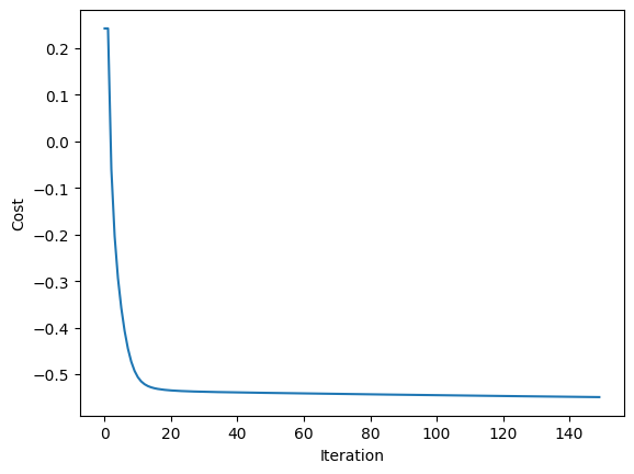
Let’s visualise the gradient descent
plt.plot(cost_vals)
plt.xlabel("Iteration")
plt.ylabel("Cost")
Text(0, 0.5, 'Cost')